Bootstrap Estimates

from magentropy import MagentroData

magdata = MagentroData('magdata.dat')
magdata.process_data()

Show code cell output Hide code cell output

"[Data]" tag detected, assuming QD .dat file.
The sample mass was determined from the QD .dat file: 0.1
The data contains the following 5 magnetic field strengths and observations per field:
20.0     100
40.0     100
60.0     100
80.0     100
100.0    100
Name: T, dtype: int64

Processing data using the following settings:
{
	npoints: 1000,
	temp_range: [-inf  inf],
	fields: [],
	decimals: 5,
	max_diff: inf,
	min_sweep_len: 10,
	d_order: 2,
	lmbds: [nan],
	lmbd_guess: 0.0001,
	weight_err: True,
	match_err: False,
	min_kwargs: {'method': 'Nelder-Mead', 'bounds': ((-inf, inf),), 'options': {'maxfev': 50, 'xatol': 0.01, 'fatol': 1e-06}},
	add_zeros: False
}

scipy.optimize.minimize: Optimization terminated successfully.
Processed M(T) at field: 20.0
scipy.optimize.minimize: Optimization terminated successfully.
Processed M(T) at field: 40.0
scipy.optimize.minimize: Optimization terminated successfully.
Processed M(T) at field: 60.0
scipy.optimize.minimize: Optimization terminated successfully.
Processed M(T) at field: 80.0
scipy.optimize.minimize: Optimization terminated successfully.
Processed M(T) at field: 100.0
Calculated raw derivative and entropy.

last_presets set to:
{
	npoints: 1000,
	temp_range: [  0.99999934 100.00000083],
	fields: [ 20.  40.  60.  80. 100.],
	decimals: 5,
	max_diff: inf,
	min_sweep_len: 10,
	d_order: 2,
	lmbds: [0.00091728 0.00054639 0.00072862 0.00091728 0.00095775],
	lmbd_guess: 0.0001,
	weight_err: True,
	match_err: False,
	min_kwargs: {'method': 'Nelder-Mead', 'bounds': ((-inf, inf),), 'options': {'maxfev': 50, 'xatol': 0.01, 'fatol': 1e-06}},
	add_zeros: False
}

Finished.

magdata.processed_df

	T	H	M	M_err	M_per_mass	M_per_mass_err	dM_dT	Delta_SM
0	0.999999	0.002	0.000002	NaN	19.847003	NaN	-0.098265	-0.000098
1	1.099098	0.002	0.000002	NaN	19.837267	NaN	-0.098240	-0.000098
2	1.198198	0.002	0.000002	NaN	19.827533	NaN	-0.098202	-0.000098
3	1.297297	0.002	0.000002	NaN	19.817803	NaN	-0.098138	-0.000098
4	1.396396	0.002	0.000002	NaN	19.808082	NaN	-0.098050	-0.000098
...	...	...	...	...	...	...	...	...
4995	99.603604	0.010	0.000001	NaN	11.673323	NaN	-0.829550	-0.004619
4996	99.702704	0.010	0.000001	NaN	11.591120	NaN	-0.829466	-0.004620
4997	99.801803	0.010	0.000001	NaN	11.508924	NaN	-0.829407	-0.004620
4998	99.900902	0.010	0.000001	NaN	11.426733	NaN	-0.829371	-0.004620
4999	100.000001	0.010	0.000001	NaN	11.344545	NaN	-0.829347	-0.004620

5000 rows × 8 columns

The problem of estimating true statistical model parameters using a single data set is commonly approached using bootstrap procedures. Given data of length \(N\), bootstrap resampling involves repeatedly sampling \(N\) points from the data with replacement, fitting a model to each of the \(N_\mathrm{B}\) data samples, and computing the parameter of interest from the \(N_\mathrm{B}\) fitted models.

In our case, we want to estimate the error at each output point of the smoothed magnetic moment. To do this, the standard deviation of each smoothed magnetic moment point is computed from the values of \(N_\mathrm{B}\) fitted models at each point. Every model is computed using a subset (again, sampled with replacement) of the original data, though the smoothed moment is evaluated at the same linearly-spaced points every time. (The output points are specified in presets as part of data processing.)

There are a few significant caveats associated with this approach. Each caveat get its own little admonition below. Please read!

Attention

The bootstrap method presented here is purely experimental and is not detailed in either of the sources listed on the homepage.

Caution

\(N_\mathrm{B}\) regularization problems must be solved for every temperature sweep taken at a particular field strength. As such, this method is computationally expensive and can take upwards of ten minutes to run on typical magnetization data, depending on the size of the data and how many models are fitted at each field.

Important

Bootstrap estimates in the context of regularization are dependent on the chosen regularization parameter \(\lambda\). These error estimates should not be viewed as “true” estimates but rather as the estimates for a given \(\lambda\). This method should only be used once the user is confident their \(\lambda\)’s are appropriate.

Caveats aside, the method is simple, if time-consuming. Two arguments are supported: n_bootstrap (the number of models to fit at each field) and random_seed (for reproducibility).

magdata.bootstrap(n_bootstrap=100, random_seed=0)

Performing bootstrap calculations...
Calculated bootstrap estimates at field: 20.0
Calculated bootstrap estimates at field: 40.0
Calculated bootstrap estimates at field: 60.0
Calculated bootstrap estimates at field: 80.0
Calculated bootstrap estimates at field: 100.0
Finished.

The error columns in processed_df are now filled:

magdata.processed_df

	T	H	M	M_err	M_per_mass	M_per_mass_err	dM_dT	Delta_SM
0	0.999999	0.002	0.000002	1.720299e-08	19.847003	0.172030	-0.098265	-0.000098
1	1.099098	0.002	0.000002	1.694624e-08	19.837267	0.169462	-0.098240	-0.000098
2	1.198198	0.002	0.000002	1.669156e-08	19.827533	0.166916	-0.098202	-0.000098
3	1.297297	0.002	0.000002	1.643916e-08	19.817803	0.164392	-0.098138	-0.000098
4	1.396396	0.002	0.000002	1.618925e-08	19.808082	0.161893	-0.098050	-0.000098
...	...	...	...	...	...	...	...	...
4995	99.603604	0.010	0.000001	2.348720e-08	11.673323	0.234872	-0.829550	-0.004619
4996	99.702704	0.010	0.000001	2.380203e-08	11.591120	0.238020	-0.829466	-0.004620
4997	99.801803	0.010	0.000001	2.411919e-08	11.508924	0.241192	-0.829407	-0.004620
4998	99.900902	0.010	0.000001	2.443854e-08	11.426733	0.244385	-0.829371	-0.004620
4999	100.000001	0.010	0.000001	2.475996e-08	11.344545	0.247600	-0.829347	-0.004620

5000 rows × 8 columns

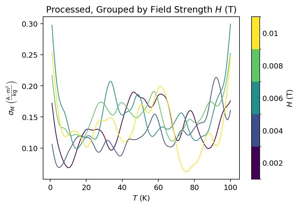
We can easily plot the errors:

import matplotlib.pyplot as plt

fig, ax = plt.subplots(figsize=(6, 4))

magdata.plot_lines(data_prop='M_per_mass_err', data_version='processed', ax=ax, colorbar=True);